This article is the first post on my TensorFlow(TF) Beginner Series. If you are looking to start out with TensorFlow then, this post and the coming once might be useful to your learning.

In this article, I'll give you a head start of the basics of TF and guide you on building your first TF model. We'll build a model that learns the training set and predicts the equivalent Fahrenheit value of a degree Celcius. This post is for an absolute Machine Learning Beginner with a basic knowledge of python and Machine Learning and with a strong mindset to learn and try out things on the fly.

What you will learn

• What TensorFlow is
• A few machine learning terminologies relevant to TF
• How to import TensorFlow2 and other relevant dependencies
• How to set up a training model
• How to create a model
• How to assemble layers in a model
• How to compile a model, with loss and optimizer functions
• How to train a model
• How to visualize model performance
• How to use the model to predict values and more.....

Gif by gifer.com

What is TensorFlow(TF)?

TensorFlow is a free and open-source software library for dataflow and differentiable programming across a range of tasks. It is a symbolic math library, and is also used for machine learning applications such as neural networks. TensorFlow is used for both research and production at Google. Wikipedia

Basic Terminologies

Before we proceed, let us take a quick recap of some machine learning terminologies that are relevant to our model in this post.

• Features - The input(s) to our model. In this case, a single value.
• Labels - The output our model predicts.
• Example - A pair of inputs/outputs used during training.
• Loss function - A way of measuring how far off predictions are from the desired outcome. (The measured difference is called the "loss").
• Optimizer function - A way of adjusting internal values in order to reduce the loss.
• input_shape=[1] - This specifies that the input to this layer is a single value. That is, the shape is a one-dimensional array with one member.
• units=1 - This specifies the number of neurons in the layer. The number of neurons defines how many internal variables the layer has to try to learn how to solve the problem (more later).
• Epoch - Specifies how many times this cycle should be run.
• Verbose - Verbose argument controls how much output the method produces

Import TF2.0 and Other Dependencies

Every typical machine learning project makes use of different dependencies or libraries specific to the subject matter. For a TF 2.0 project, you will need to first import or upgrade your old version of TensorFlow to the updated version. The few lines of code below will do the magic for you:

try:
     %tensorflow_version 2.x
except Exception:
     pass

import tensorflow as tf

Other dependencies take the usual form

import numpy as np

We only need numpy for this project.

Set up a Training Model

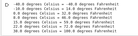
The output of every machine learning model is based on the training set (data) fed into it during the training process. Let's create two lists cel_values and fah_values to train our model.

cel_values    = np.array([-40, -10,  0,  8, 15, 22,  38],  dtype=float)
fah_values = np.array([-40,  14, 32, 46, 59, 72, 100],  dtype=float)

for i,c in enumerate(cel_values):
  print("{} degrees Celsius = {} degrees Fahrenheit".format(c, fah_value[i]))

Output:

Create a Model

Since our problem does not involve much logic, we'll use a Dense Network that requires a single layer with a single neuron.

Let us create a layer l1 and instantiate it with tf.keras.layers.Dense and the input and input_shape parameters.

 layer = tf.keras.layers.Dense(units=1, input_shape=[1])

Assemble Layers in into a Model

After defining your layers, the next step is to assemble them into your model. The Sequential model definition takes a list of layers as an argument, specifying the calculation order from the input to the output.

Note, our model has just a single layer l1

model = tf.keras.Sequential([l1])

We can combine the above command into a single command this way:

model = tf.keras.Sequential([
  tf.keras.layers.Dense(units=1, input_shape=[1])
])

Compile a Model, with Loss and Optimizer Functions

We compile our model before proceeding with the training

model.compile(loss='mean_squared_error',
              optimizer=tf.keras.optimizers.Adam(0.1))

During training, the optimizer function is used to calculate adjustments to the model's internal variables. The goal is to adjust the internal variables until the model (which is really a math function) mirrors the actual equation for converting Celsius to Fahrenheit.

TensorFlow uses numerical analysis to perform this tuning, and all this complexity is hidden from you so we will not go into the details here. What is useful to know about these parameters are: The loss function (mean squared error) and the optimizer (Adam) used here are standard for simple models like this one, but many others are available. It is not important to know how these specific functions work at this point.

One part of the Optimizer you may need to think about when building your own models is the learning rate (0.1 in the code above). This is the step size taken when adjusting values in the model. If the value is too small, it will take too many iterations to train the model. Too large, and accuracy goes down. Finding a good value often involves some trial and error, but the range is usually within 0.001 (default), and 0.1

Train the Model

Train the model by calling the fit method.

During training, the model takes in Celsius values, performs a calculation using the current internal variables (called "weights") and outputs values that are meant to be the Fahrenheit equivalent. Since the weights are initially set randomly, the output will not be close to the correct value. The difference between the actual output and the desired output is calculated using the loss function, and the optimizer function directs how the weights should be adjusted.

This cycle of calculate, compare and adjust is controlled by the fit method. The first argument is the inputs, the second argument is the desired outputs. The epoch's argument specifies how many times this cycle should be run, and the verbose argument controls how much output the method produces.

train = model.fit(cel_values, fah_values, epoch = 500, verbose = False)

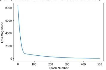
Display Training Statistics

The fit method returns a history object. We can use this object to plot how the loss of our model goes down after each training epoch. A high loss means that the Fahrenheit degrees the model predicts are far from the corresponding value in fah_value

We'll use Matplotlib to visualize this (you could use another tool). As you can see, our model improves very quickly at first and then has a steady, slow improvement until it is very near "perfect" towards the end.

import matplotlib.pyplot as plt
plt.xlabel('Epoch Number')
plt.ylabel("Loss Magnitude")
plt.plot(train.train['loss'])

Output:

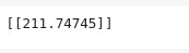
Use the model to Predict Values

Now you have a model that has been trained to learn the relationship between cel_value and fah_value. You can use the predict method to have it calculate the Fahrenheit degrees for a previously unknown Celsius degrees.

print(model.predict([100]))

Output:

Let's look a the internal variables of the dense layer

print(layer.get_weights()))

Output:

The first variable is close to ~1.8 and the second to ~32. These values (1.8 and 32) are the actual variables in the real conversion formula.

This should give you a good headstart of the workflow of TensorFlow. In the coming posts, we'll explore more advance case studies and get you up to speed with different TF techniques.

Find the complete code for this post on my Github Repo

Citation: Udacity:Intro to TensorFlow for Deep Learning Course

Further Read:

TensorFlow Official Site